Metric learning aims to learn an embedding space, where the embedded vectors of similar samples are encouraged to be closer, while dissimilar ones are pushed apart from each other. Multi Similarity Loss proposed intuitively better methods to achieve this and is backed up by its accuracies across public benchmark datasets. This paper main contribution are two fold: a) Introducing multiple similarities into the mix, b) hard pair mining.
Multiple Similarities:
This loss deals with 3 types of similarities that carry the information of pairs.
1. Self Similarity:
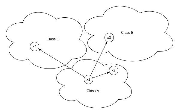
Self similarity ensures that instances belonging to positive class remains closer to anchor than the instances associated with negative classes.
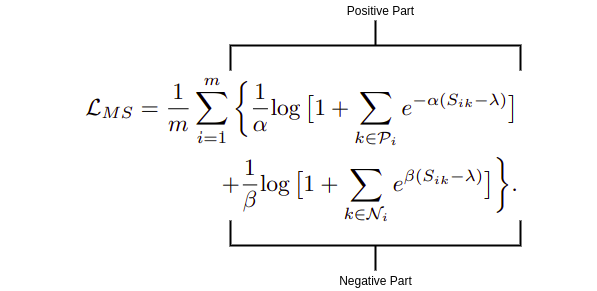
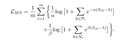
Ms-Loss comprises of two parts:
i) Positive Part:
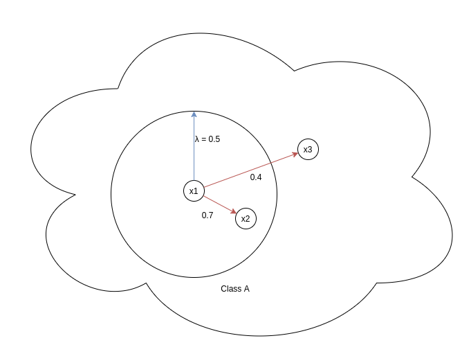
This part deals exclusively with p-pairs (positive pairs). λ represents the similarity margin which controls the closeness of p-pairs by heavily penalizing those p-pairs whose cosine similarity < λ. In the above diagram we can see two pairs x1-x2 and x1-x3, positive part of the loss for x1-x2 would be very low since e^(-α(Sᵢₖ — λ)) = e^(-α(0.7–0.5)) = e^(-0.2 * α), since α is hyperparameter and always greater than zero, value of this term will be very low when compared with positive part of the loss for x1-x3. For this pair, loss will be e^(-α(0.4–0.5)) = e^(0.1 α)). Cleⱼar distinction is there between the loss back propagated for x1-x2 and x1-x3.
ii) Negative Part:
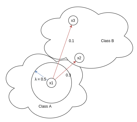
This part deals exclusively with n-pairs (negative pairs). This part of the loss ensures negatives to have as low as possible similarity with the anchor. This means that negatives lying closer to x1 ( i.e having high similarity) should be penalized heavily than negatives lying further away from x1 ( i.e having low similarity). This is evident from the loss, for eg. loss for x1-x2 is e^(β(Sᵢₖ — λ)) = e^(β(0.3–0.5)) = e^(-0.2 * β), whereas loss for x1-x3 is e^(β(0.1– 0.5)) = e^(-0.4 * β), since e^(-0.2 * β) > e^(-0.4 * β) for β > 0,hence loss for n-pairs with high similarity will be more than n-pairs with low similarity.
2. Negative relative similarity:
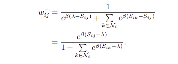
Maths for the above eq. will be shared in another Blog. Weight wᵢⱼ for a pair is defined as contribution of loss from that pair towards the total loss.
Taking into consideration only one n-pair x1-x2, ms-loss not only assign weight to this pair only on the basis of self-similarity between x1-x2 but also on the basis of its relative similarity i.e all other negatives present in the batch with respect to x1.
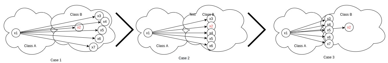
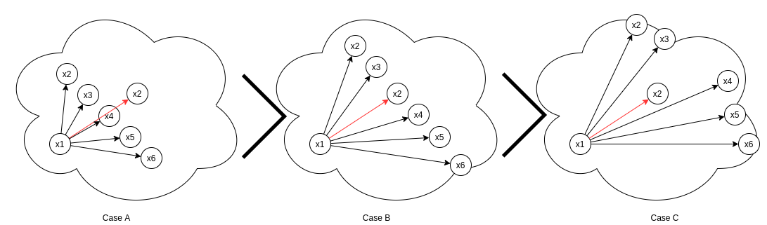
In the above eq. Sᵢⱼ refers to self similarity between x1-x2 and Sᵢₖ refers to similarity between x1-x3,x1-x4,x1-x5,x1-x6,x1-x7. In the above image though x1-x2 has same similarity Sᵢⱼ across all cases, its w-ᵢⱼ varies across cases.
- Case 1: All other negatives (x3,x4,x5,x6,x7) are farther away from x1 with respect to x2.
- Case 2: All negatives (x2,x3,x4,x5,x6,x7) lie at an equal distance from the anchor x1.
- Case 3: All other negatives (x3,x4,x5,x6,x7) lie closer to x1 with respect to x2.
- Case 1: w-ᵢⱼ is highest, since denominator term Σ[e^(β(Sᵢₖ- Sᵢⱼ))] is lowest as all Sᵢₖ<Sᵢⱼ making this e^(negative term)
- Case 2: w-ᵢⱼ is in middle, since in denominator term Σ[e^(β(Sᵢₖ- Sᵢⱼ))], Sᵢₖ≃ Sᵢⱼ making it e^(zero-ish term).
- Case 3: w-ᵢⱼ is lowest, since denominator term Σ[e^(β(Sᵢₖ- Sᵢⱼ))] is largest as all Sᵢₖ>Sᵢⱼ, therefore making this e^(positive term).
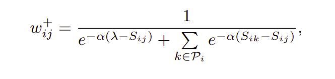
Negative relative similarity states the relationship of a single negative pair with all other negative pairs in the batch. Similarly positive relative similarity defines the relation between a single positive (x1-x2)and all other positives(x1-x3,x1-x4,x1-x5,x1-x6) in the batch. Following the procedure we did under Negative relative similarity heading, we can easily verify the results stated in the above image.
Mining Hard Positives And Negatives
Authors of Multi-Similarity loss paper used only hard negatives and positives for training and discarded all other pairs as they contribute little to no improvement and sometimes degraded the performance as well. Choosing only those pairs that carries the most information also make the algo computationally faster.
i) Hard Negative Mining:
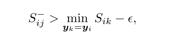
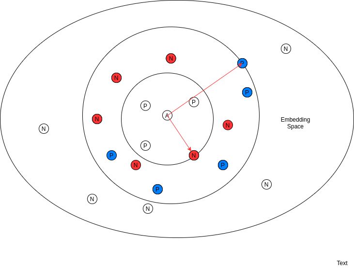
The above eq. states that only those negatives should be included in training whose similarity with the anchor is greater than minimum similarity of a positive (positive which is lying furthest in embedding space). Therefore in the above diagram only negatives we have chosen are the red ones since they are all lying inside the positive with minimum similarity to anchor, rest all negative are discarded.
ii) Hard Positive Mining:
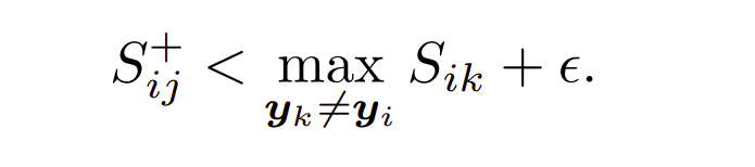
The above eq. states that only those negatives should be included in training whose similarity with the anchor is less than maximum similarity of a negative (negative lying closest to anchor). Hard positives are coloured blue while rest are discarded.
Understanding the code
class MultiSimilarityLoss(nn.Module):
    def __init__(self, cfg):
        super(MultiSimilarityLoss, self).__init__()
        self.thresh = 0.5
        self.margin = 0.1
        self.scale_pos = cfg.LOSSES.MULTI_SIMILARITY_LOSS.SCALE_POS
        self.scale_neg = cfg.LOSSES.MULTI_SIMILARITY_LOSS.SCALE_NEG
    def forward(self, feats, labels):
        # feats = features extracted from backbone model for images
        # labels = ground truth classes corresponding to images
        batch_size = feats.size(0)
        sim_mat = torch.matmul(feats, torch.t(feats))
        # since feats are l2 normalized vectors, taking
its dot product with transpose of itself will yield a similarity matrix whose i,j (row and column) will correspond to similarity between i'th embedding and j'th embedding of the batch, dim of sim mat = batch_size * batch_size. zeroth row of this matrix correspond to similarity between zeroth embedding of the batch with all other embeddings in the batch.
        epsilon = 1e-5
        loss = list()
        for i in range(batch_size):
            # i'th embedding is the anchor

            pos_pair_ = sim_mat[i][labels == labels[i]]
            # get all positive pair simply by matching ground truth labels of those embedding which share the same label with anchor
            pos_pair_ = pos_pair_[pos_pair_ < 1 - epsilon]
            # remove the pair which calculates similarity of anchor with itself i.e the pair with similarity one.
            neg_pair_ = sim_mat[i][labels != labels[i]]
            # get all negative embeddings which doesn't share the same ground truth label with the anchor
            neg_pair = neg_pair_[neg_pair_ + self.margin > min(pos_pair_)]
            # mine hard negatives using the method described in the blog, a margin of 0.1 is added to the neg pair similarity to fetch negatives which are just lying on the brink of boundary for hard negative which would have been missed if this term was not present.

            pos_pair = pos_pair_[pos_pair_ - self.margin < max(neg_pair_)]
            # mine hard positives using the method described in the blog with a margin of 0.1.
            if len(neg_pair) < 1 or len(pos_pair) < 1:
                continue
            # continue calculating the loss only if both hard pos and hard neg are present.
            # weighting step
            pos_loss = 1.0 / self.scale_pos * torch.log(
                1 + torch.sum(torch.exp(-self.scale_pos * (pos_pair - self.thresh))))
            neg_loss = 1.0 / self.scale_neg * torch.log(
                1 + torch.sum(torch.exp(self.scale_neg * (neg_pair - self.thresh))))
            # losses as described in the equation
            loss.append(pos_loss + neg_loss)
        if len(loss) == 0:
            return torch.zeros([], requires_grad=True)
        loss = sum(loss) / batch_size
        return loss
Resources
Official Github implementation: https://github.com/MalongTech/research-ms-loss/blob/master/ret_benchmark/losses/multi_similarity_loss.py
If you are passionate about deep learning, or simply want to say hi, please drop me a line at [email protected]. Any suggestion regarding the blog will be great as well. www.linkedin.com/in/kshavG